 Overview
This page is an overview of the work I have taken part in involving ROS.
Robot Specific ROS Nodes
This section discusses the ROS nodes that are generally required to ROSify a robot. Not all of these apply to each robot, though this setup was taken from ROS wiki documentation, tutorials, and support packages for well-established robots like the Turtlebot series.
Robot Description
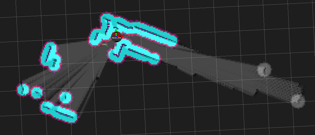
One of the foundations of ROS functionality is the TF library, or the transform library. This allows an easy method for transforming between various frames of reference. For instance, the ground on which our robot will always be a static frame of reference as it never moves. However, our robot with wheels can move along the ground changing position and orientation with respect to the ground. If one intends to draw a map using only data from the robot, the current transformation from the ground frame to the robot’s frame must be known.
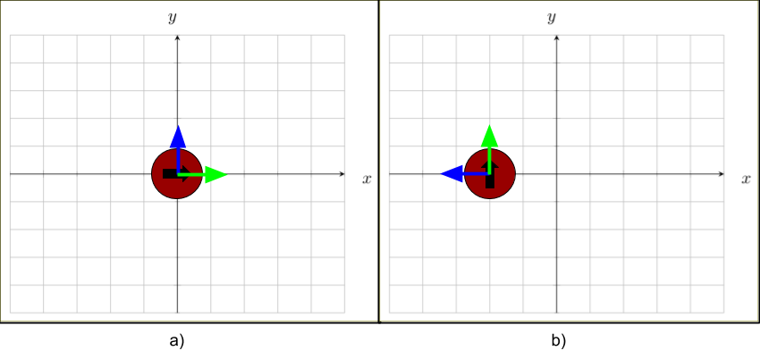
The simple grids above show two examples of how the robot’s frame, marked by the red circle, can change with respect to the static ground frame, denoted by the grid. The robot’s orientation is denoted with the green (positive X) and blue (positive Y) axes. In grid a), the robot orientation is centered at the origin and its orientation inline with the ground frame, thus no transformation is needed to change between frames. In grid b), the robot has moved to position (-2,0) on the map grid and has also turned 90 degrees counterclockwise. Here, we must apply a translation and rotation to change between the map and robot frame.
ROS transformations allow for translations and rotations in the X, Y, and Z dimensions.
In order to effectively apply transformations and quickly change between frames, ROS allows for a robot model or description to be given as URDF file of links and joints. Links are physical structures of the robot such as the wheel, while joints denote connections between links, such as the axle joint connection the wheel and robot frame links. This description must be in the form of a valid TF tree such that every child link must have only a single parent link.
With a given robot description, the ROS package robot_state_publisher will handle the broadcast of the current robot state to the TF library, thus ensuring the appropriate transform is available when needed to all ROS nodes.
For the Arlo Autonomous Ground Vehicle, the primary transformations needed are from the laser scanner frame to the robot base frame, both wheel frames to the robot base frame, and lastly, the robot base frame to the static map frame or ground. The former two are static as the laser and the wheels are both mounted to the robot base frame. The final robot base frame to map frame transformation can be determined by dead-reckoning odometry from wheel encoders or more sophisticated odometry methods using the laser scanner.
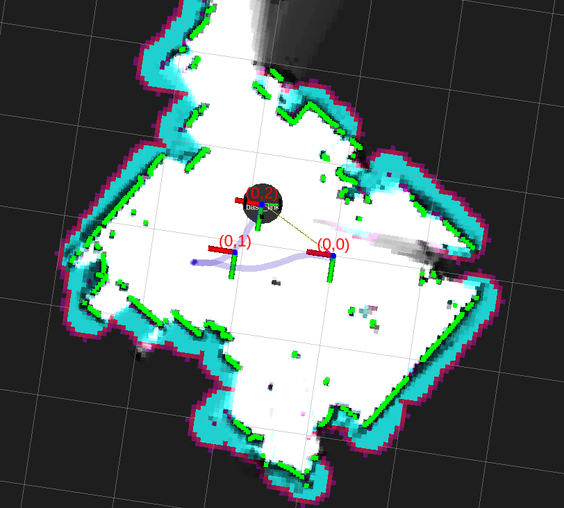
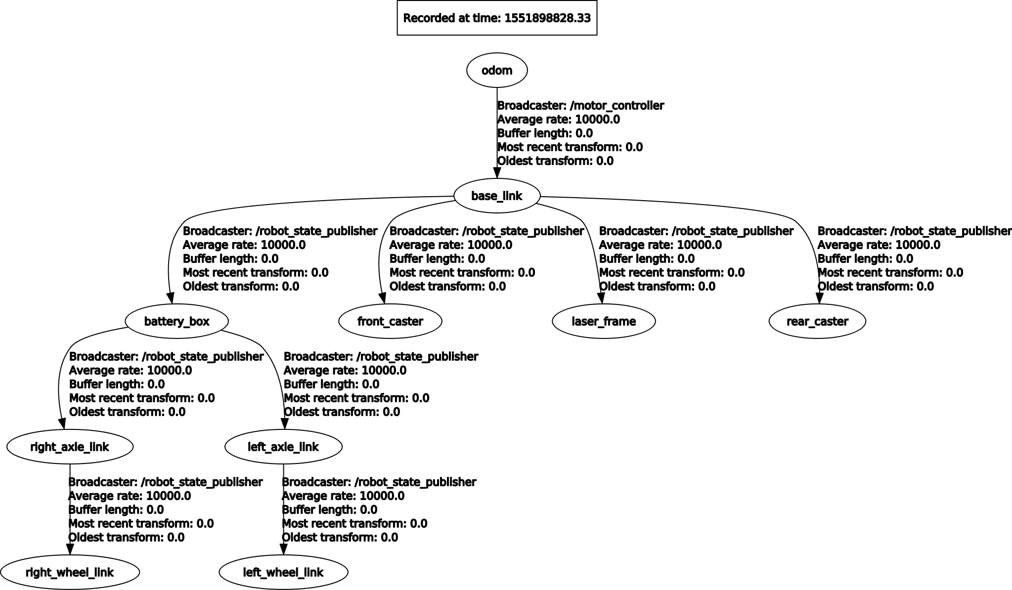 This local TF tree denotes the relationships written in the robot description URDF file. In addition, it shows the odometry frame that is not listed in the URDF file and is served by our joint interface for the Arlo robot, the motor_controller node.
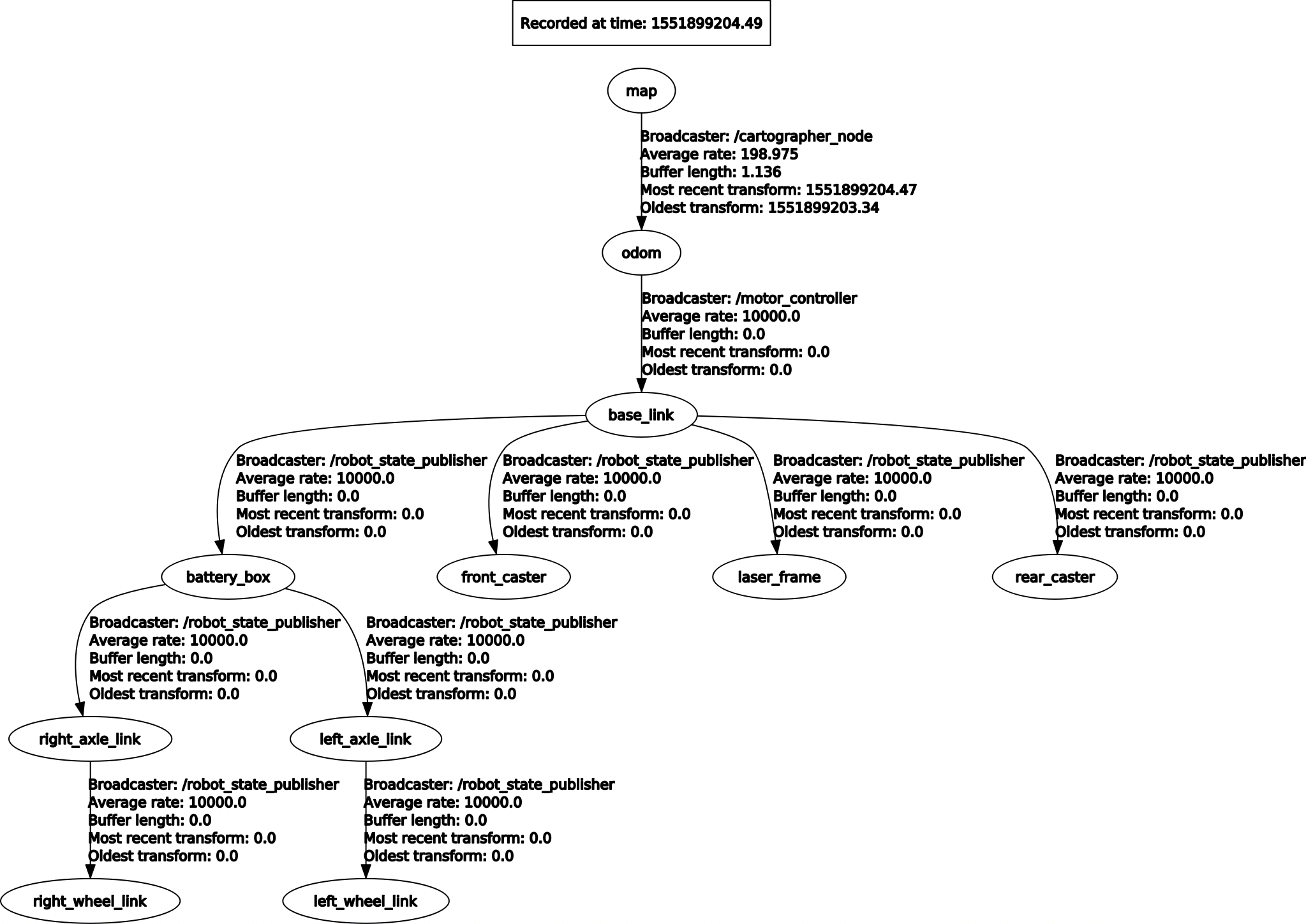 This global TF tree additionally adds the map frame. Note the map frame is not given in the URDF file and is, in our case, intended to be served by a ROS node that builds a map such as Google Cartographer.
Odometry
As can be seen in the Global TF tree above, the primary parent is the map frame with a single child, the odometry frame. The robot description tree is itself a child of the odometry frame, thus the ability to localize the robot and its peripherals in the environment is dependent on the accuracy of the map to odometry transformation.
One option mentioned above is dead reckoning. This essentially only utilizes the robots odometry from encoder readings for the map to odometry transform. As with any physical system, there will be error in these readings and solely depending on these reading would introduce this error into the ROS aware path of the robot.
Another option is odometry calculated from laser scans. Lidar range finders can provide one, two, or three-dimensional point maps that will be altered as the robot moves through the environment. However, this requires a bit more complexity and is typically available in ROS packages for SLAM and other mapping techniques. See below for a description of our implementation with Google Cartographer on the Arlo Autonomous Ground Vehicle.
Joint Interface
ROS describes structural components of robots with links and joints, where links are physical structures attached to others via joints. Joints can be static in the case of a hard mounted laser scanner or dynamic in the case of axles attaching wheels to a robot body.
In order to control the a ROS robot, there must be some controller for each dynamic joint. In the case of the Arlo Autonomous Ground Vehicle, we have implemented a simple motor controller interface to control the motor speeds and runs as a ROS node. Considering these motors control our robot’s locomotion, we also subscribe to the typical cmd_vel message for retrieving the appropriate speed to issue to the physical motor controller board.
Mobility
The kinematics of any robot will be slightly different than others. Does the robot move via wheeled locomotion or legged? Both produce drastically different setups but each still would typically use the cmd_vel message to retrieve commands for movement. The cmd_vel message is composed of linear and rotational velocities that must be converted to appropriate joint commands.
For the Arlo Autonomous Ground Vehicle, we must depend on the kinematics of a wheeled non-holonomic robot. It has two wheels centered on outsides of the round structural frame, thus it cannot move sideways and only forwards, backwards, or rotational motion is available. Please refer to the Arlo Autonomous Ground Vehicle page for equations.
RPLidar A1
We use the RPLidar A1 on the Arlo Autonomous Ground Vehicle to produce two-dimensional point-maps. The ROS package rplidar for handling the interaction with the laser scanner and retrieving a LaserScan message.
Google Cartographer
A predominant library for realtime two-dimensional or three-dimensional SLAM is Google Cartographer. This library has been made available to the ROS ecosystem with the cartographer-ros package.
Simultaneous Localization and Mapping (SLAM)
We have chosen this library as the sole package for handling SLAM for the Arlo Autonomous Ground Vehicle. Cartographer allows for both realtime and offline map building, though seeing as the goal for the Arlo robot was autonomous exploration in an unknown environment, we have worked primarily with realtime scenarios.
This package can subscribe to robot odometry and the laser scans in order to orient itself, collecting scans, can subsequently build a map via matching successive scans.
I would like to go deeper into my current configuration of cartographer for the Arlo robot, but there are many settings I am still playing with for better made maps.
Move Base
The move_base ROS package is provided as an implementation of ROS actions (see actionlib). Actions are simply preemptable tasks such as moving to an environmental target location. The move-base package simply attempts to complete the requested action.
With actions such as providing a navigation goal, a local and global planner are both used to build a path in order to reach the target. In our case, we have used move_base as the controller for navigating a Google Cartographer built two-dimensional map with the Arlo robot. Given our perception of the environment is limited to two-dimensions, we utilize two, two-dimensional costmaps generated by the local and global planners.
The pink and blue areas represent areas with an assigned cost. Settings for adding sensor readings to the costmaps can be adjusted with the planner configurations. Here we only detect obstacles in the underlying map that are within the set thresholds. This is purposely a poorly generated map to demonstrate the difference between the global map and costmaps.
The map denoted by the grayscale filling is much whiter in this image as the mapping has had sufficient sensor readings to rate these areas with high confidence. In turn, the obstacles denoted by the blue and pink costmaps are finer tuned as a result of this map confidence.
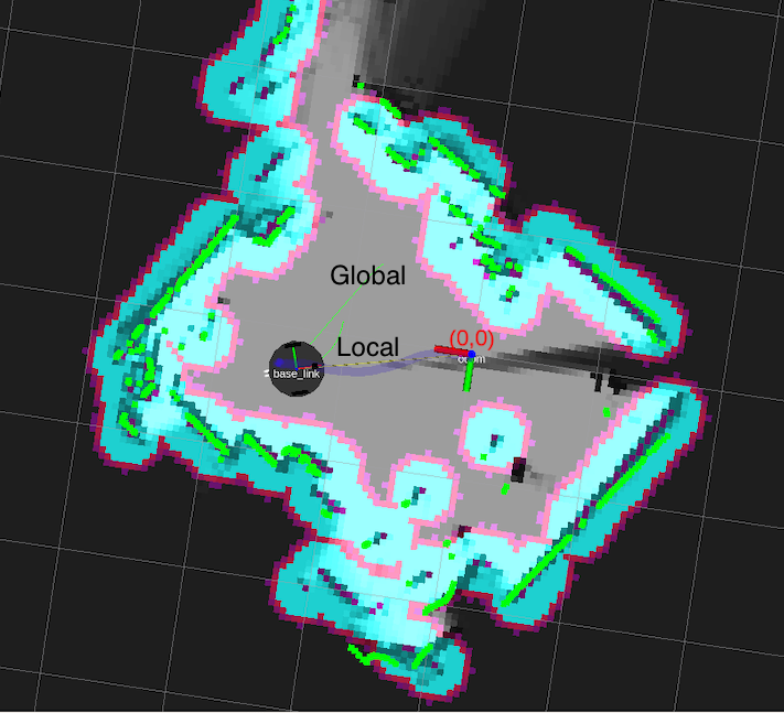
The paths are denoted by the green lines marked global and local extending from the base of the robot. These paths are different as the local planner must also consider the current robot’s orientation and if the robot is reacting to the velocity commands in the expected manner. In this image, the local planner is attempting to reach the global path as quickly as possible by making a left turn. The global planner acts similarly though operates under different parameters and a larger window of the map is used.